Properties of Projectiles

Overview:
We started a new unit with an introductory experiment. The experiment was simply to throw a ball forward and upward, and take a video. From there, we uploaded the video to a program called PascoCapstone. We tracked the ball's motion while in the air and then were able to find some key characteristics of projectile motion. The main thing that we discovered was that the motion in the horizontal direction is completely independent from the motion in the vertical direction.

Graphs/Raw Data:

This image shows the path of the ball that we threw. The red plus signs show the position of the ball. 

This graph shows the position of the ball vs the time. The red line is the horizontal displacement, and the green line is the vertical displacement.

This graph shows the velocity of the ball vs. the time. The pink line shows the velocity of the Y-axis. The blue line shows the velocity of the X-axis.

Analysis of Data:
With the information that these graphs have given, we can manipulate the data to find certain unknowns.

Acceleration in y axis: 9.8m/s^2 -- We know this because on earth the force of gravity is always the same.
Acceleration in x axis: 0 m/s^2 -- We know this because there is no unbalanced force to accelerate the ball in the horizontal direction. It is at constant velocity.

Initial velocity in y: ~2.1m/s -- We know this because its the y intercept of the vertical plane
Initial velocity in x: 3.88m/s -- We know this because it is the y-intercept for the horizontal plane

Velocity at the top of the path on y axis: 0m/s^2 -- We know this because the ball is changing direction and stops momentarily.
Velocity at the top of the path on x axis: 3.8m/s -- constant velocity

Final Velocity in x: 2.2 m/s -- final point on v vs. t graph
Final Velocity in y: -0.5m/s -- final point on v vs. t graph

How High the ball got: 2.53m -- we can look on the x vs. t graph
How far the ball went: 3.05m -- I used Xfinal - Xinitial = Change in X

Time for the ball to reach the top of its path: 0.835s -- Used equation Vf=at+Vi
Total air time for ball: 1.57s -- x=1/2at^2+vit

Conclusions:
In this experiment, we learned that the vertical and horizontal motions are completely unrelated when dealing with projectiles. We also discovered that all horizontal motion was constant, so we could use formulas and equations from the BFPM unit. The vertical motion was all constant acceleration; we used the UFPM equations. The same principle applied for solving for displacement. The horizontal motion remained constant for the entire trip and the vertical motion stopped at the top of the path. Furthermore, we were able to use the graphs that we created to find many of the unknowns, which proved to be helpful.

UFPM Practicum Lab

Goal:
The purpose of this lab was to test our knowledge of unbalanced forces and our applied use of kinematics. We demonstrated these skills with this lab. Our goal was to try and land a weight attached to a cart on another cart below going at constant velocity.

Procedure:
We first found the mass of the entire system. 0.693kg (We rounded to .64kg)

We then solved for acceleration. (The weight was .5N)

a=Fnet/m

a=.5N/.64kg

a=0.78m/s^2

After, we found the distance from the starting position of the weight to where it would land on the cart. The distance was .74m.

Using the information that we now had, we were able to solve using a formula for time.

x=1/2at^2+Vit

(.74)=1/2(.78)(t)^2

1.89=t^2

t=1.37s

Next, using the formula V=(change in)x/(change in)t we found the velocity of the cart on the ground. We concluded that the cart went 1 meter in 3.6 seconds. We manipulated these numbers to find that the cart had a constant velocity of .28m/s. Using these equations we hypothesized that if we placed the constant velocity cart 0.38m away from the weight. We could release both at the same time and the weight would land on top of the cart.

After our initial test, we proved our hypothesis correct and were able to land the weight perfectly on top of the cart.

We filmed our test which can be seen HERE.

Fan Car Acceleration Experiment

Overview: 
The purpose of this lab was to take two fan powered cars with different accelerations going in different directions, and try and predict where and when they would collide. 

Materials: 

• Fan Powered Car
• Stop Watch
• Meter measuring stick
• chalk

Procedure:

We started the lab by finding the acceleration of our car. We did this by marking the displacement of the car at each second of motion. We then shared our data with another group so we could calculate the point of intersection. Once we compared data, we manipulated the accelerations to find where and when the two cars would collide. 

Raw Data:

Time       Their Data    Our Data

Manipulated Data:

Here is the position vs time graph for the two cars

Summary: 

We collaborated with Miranda and Morgan's group to find the position and time of intersection. They were our partner group, so we were able to use the same test and the same numbers as them. We ended up being within the allowed 5% error margin at the end of the experiment. 

Prediction: 

Time: ~2.5 seconds 

Position: ~61 cm

Actual: 

Time: 2.9 seconds

Postion: 63 cm

Forces: Challenge Lab

Introduction:
In this lab, we tried to find the weight of an object based on the tension of the wire that was holding it up.

Data:
We used trigonometric ratios to find the unknown tensions.

FBD for the experiment

Cos58 = fty1 / 1.6

-> fty1 = 0.85N

Cos22 = fty2 / 3.5

-> fty2 = 3.25N

With these tensions, I concluded that the weight of the object must have been 4N. I was correct.

Unit 3 Summary: CAPM

Introduction:
This unit, our class learned about constant acceleration, and created the Constant Velocity Particle Model. 

Instantaneous Velocity:
1. The first way of finding the instantaneous velocity is to determine the slope of the tangent to an x vs. t graph at a given point. 

2. The second way is to use the mathematical model:
vf=at+vi
(Final Velocity = acceleration * time + Initial Velocity)

Two graphs depicting velocity vs. time and position vs. time

Displacement: 
1. The first way of finding the displacement of an object is to find the area under a V vs. T curve. This process is demonstrated in the V vs T graph above. 

2. The second way is to use the mathematical model:
x = 1/2at^2 + vit
(positon = 1/2 acceleration * time squared + initial velocity * time)

Acceleration:
1. The first way of finding the acceleration of an object is to find the slope of a v vs. t graph

2. Using the mathematical model:
a = change in v / change in t

3. Solving for acceleration in the mathematical model:
x = 1/2at^2 + vit
(positon = 1/2 acceleration * time squared + initial velocity * time)

4. Solving for acceleration in the mathematical model:
vf=at+vi
(Final Velocity = acceleration * time + Initial Velocity)

x vs. t graphs:
1. With a position vs. time graph, you can find the starting position, direction of motion, and velocity. You can also use the graph to draw a v vs. t graph or an a vs. t graph.
2. You can use the information to draw a motion map
3. You can determine the average and instantaneous velocity (as mentioned above).
4. You can determine the displacement (as mentioned above)

The x vs. t graphs are showing constant acceleration

v vs. t graphs:

1. With a velocity vs. time graph, you can find the acceleration (explained above), and find the direction of motion (positive or negative slope). 

2. You can use it to draw an x vs. t graph

3. You can use it to draw an a vs. t graph

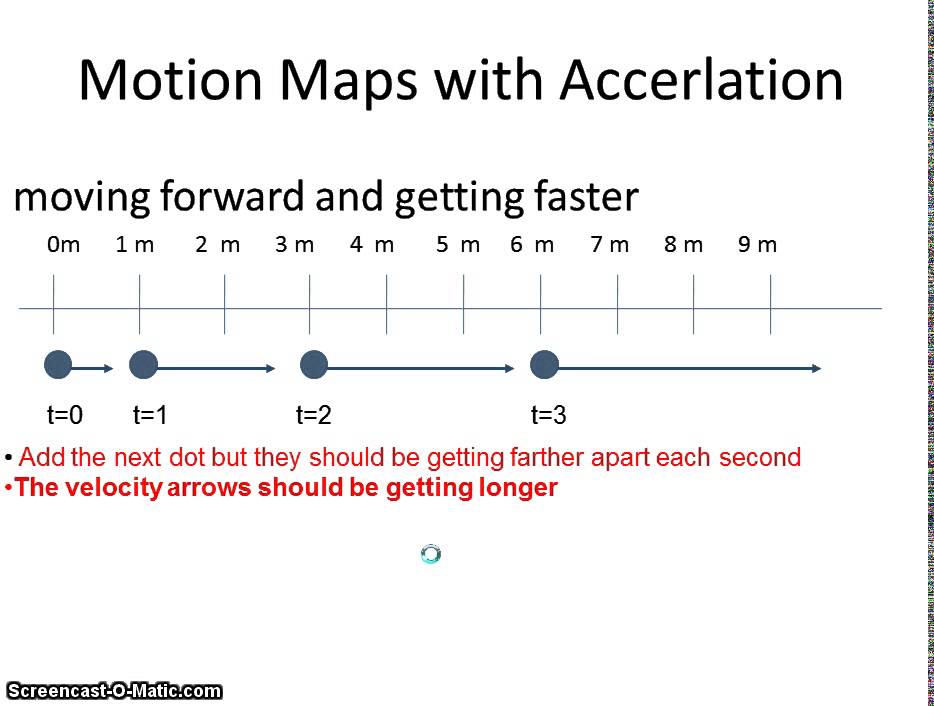
4. You can use it to draw a motion map (with velocity and acceleration vectors

Motion map showing constant acceleration

CAPM Challenge - Rolling Ball Acceleration

Introduction:
For this challenge, our physics class was tasked with finding the acceleration of a ball rolling down a table. We were allowed to use a ball, chalk, and a ruler. We also had to fined the instantaneous velocity of the ball at 4 seconds.

Procedure:
We are going to have a ball on the table(inclined). We will mark the position of the ball at each half second with the chalk and will measure with the ruler. We predicted that there will be a constant acceleration of the ball.


Raw Data:
This data came from an average of three trials, and is converted from originally cm to m.

Time(s)     Position(m)
.5               .056
1                .148
1.5             .283
2                .466
2.5             .682
3                .905

Evaluation of Data:
Originally, we found the x vs. t graph, but we changed it to be x vs. t^2 because that linearized the graph and gave us the equation for the line. We used this data to find the acceleration of the ball. Our equation from the x vs. t^2 Graph was:
Position=.0973(time)+.0546
We were able to use this equation to find our predicted acceleration of the ball.
Acceleration = 0.1946 m/s^2

This graph shows the position vs. time^2 graph after we manipulated the data

This graph shows the position vs. time from our raw data.

Conclusions:

From this lab we have used our learning from class, and applied it to the real world. We took data using only a ball, a ruler and chalk, and were able to calculate the acceleration of the ball. Our error margin was within ten percent also, which shows our knowledge of this material.

Unit 2 Summary: Forces

Introduction and Newton's First Law:
We started this unit with an experiment where we rode on a hovercraft and pushed bowling balls with brooms. While these experiments were fun, they also taught us about the topic of our upcoming unit: Forces. Our class began by riding on the hovercraft. We quickly realized that once we were in motion, we kept moving at a constant velocity until someone stopped us. There were no forces acting on us when we were on the hovercraft. The same principles applied to the bowling ball experiment. We began by pushing the ball with a broom, and we found that the ball would keep rolling indefinitely unless we changed its direction or stopped it with the broom. These two experiments demonstrated Newton's First Law. 

Newton's First Law:
An object will remain at rest or in uniform motion in a straight line unless acted upon by an external force. It may be seen as a statement about inertia, that objects will remain in their state of motion unless a force acts to change the motion.

Free Body Diagrams:
One of our new models that we developed over the course of the unit was the free body diagram. This diagram shows the direction of all forces acting on an object. If the object is moving at constant velocity or is at rest, the two opposite forces will be equal. If the object is gaining speed, losing speed, or changing direction, the forces will be unbalanced. The forces will also appear on an x and y axis. 

The Free Body Diagram pictured above is balanced,
meaning it is at constant velocity or at rest. 

Types of Forces:

Gravity: The force pulling objects to the center of the earth

Normal Force: The force opposing the force of gravity, it pushes

away from the earth.

Push Force: The force of one object pushing another.

Friction: The force of an object dragging. It can only be as strong as the force that it is opposing.

Tension Force: The force along a rope.

Spring Force: The elasticity of a spring; how much a spring wants to return to its original form. 

Real World Application:

This example shows a climber on the side of a mountain, repelling down. The forces in this example are the force pull or tension on the rope and the force gravity in the vertical direction. Also, the climber has his foot against the mountain which is creating a friction force that opposes the force of gravity. There is a normal force on his foot from the mountain. 

Force Formulas:
The first formula that we learned was for converting between Mass and weight

W=MG

The W in the equation is for weight (expressed in Kg). The M is for Mass (expressed in Newtons). The G is for gravity (Newtons), and it is equal to 10N. 

The second formula we learned was for calculating the friction of an object.

Newton's Third Law:

The final law that we learned was Newton's Third Law. It states that for every action there is an equal and opposite reaction. This means that there is always a pair of forces acting oppositely on two interacting objects. For example if a someone pushes a table across the room, the table also pushes the person with equal force.